
A chemical dosing system can deliver the specified flow rate while still leaving an uneven concentration across the pipe. For an engineer, the useful question is where the mixture becomes sufficiently uniform for the next stage of the process. That location may be some distance beyond the mixer itself.
In a Graphler Technology Solutions project, we used Computational Fluid Dynamics (CFD) to evaluate a 100 NB static mixer handling water and a sodium hypochlorite solution. The analysis followed the mixture through the mixer and along the downstream pipe. It showed that concentration uniformity continued to improve after the fluid left the mixing elements.
Following the mixture through the complete flow path
The model included the static mixer and a 3.4 m pipe arrangement. Water entered at 20.8 m³/h, while a 7.5% sodium hypochlorite solution entered through the dosing inlet at 23.3 litres per hour. These conditions defined the specific case evaluated.
We examined velocity and solution volume fraction on longitudinal sections and at cross-sectional planes. The selected planes included a location upstream of the mixer, a section 100 mm beyond the mixer end, a further downstream section and the outlet. This allowed the study to distinguish what happened inside the mixing zone from what developed along the pipe.
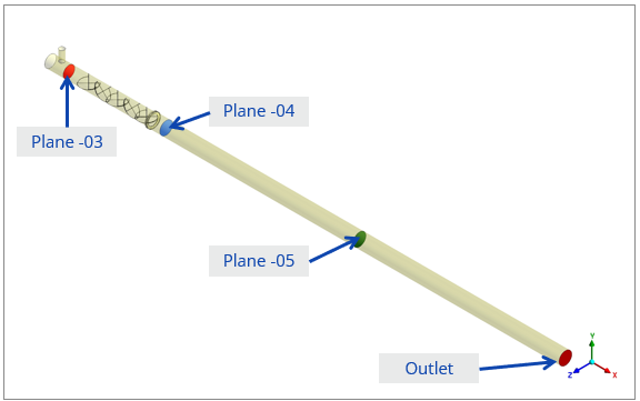
Figure 1. CFD model and sampling planes used to follow mixing through the static mixer and downstream pipe.
Measuring uniformity across the pipe
The study used the coefficient of variation, or CoV, to describe how much the solution volume fraction varied across each sampled section. A lower CoV indicates a more uniform distribution. This metric provides a numerical counterpart to the concentration contour plots, which show where richer and leaner regions remain.
A concentration average alone cannot reveal that pattern. Two sections can have similar averages while distributing the solution differently across their area. Reviewing the contours alongside CoV makes the assessment more useful for decisions about downstream equipment and sampling locations.
What the CFD results showed
At 100 mm downstream of the mixer, the report recorded a CoV of 7.22% and classified the mixture as moderately mixed. At the model outlet, the reported CoV was approximately 0.04%, classified as a good mix. The outlet contour also showed a much more even solution distribution.
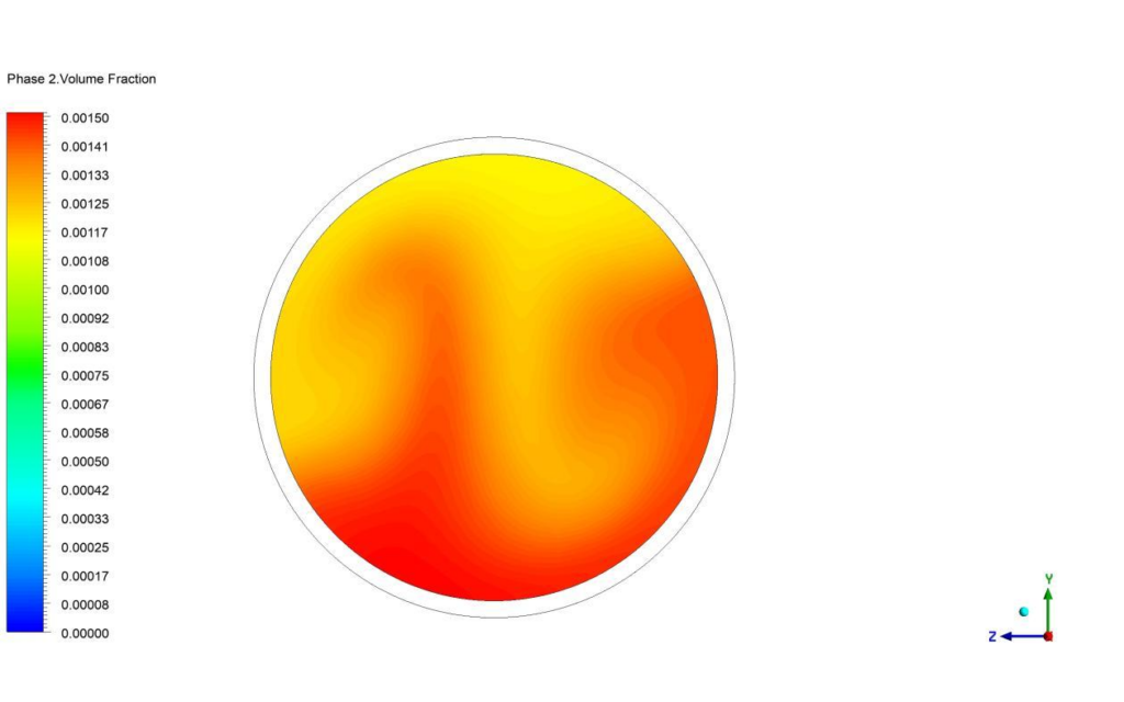
Figure 2. Solution volume fraction 100 mm beyond the mixer on the left and at the outlet on the right. Both plots use the same colour scale.
| Evaluation location | Reported CoV | Report classification |
| 100 mm beyond mixer | 7.22% | Moderate mix |
| Model outlet | 0.04% | Good mix |
These are predictions at two locations within the same simulated configuration. The difference shows the importance of downstream mixing development; it does not represent a comparison between an original and a redesigned mixer. The 0.04% value describes spatial variation in the solution distribution, not the chemical dose or a treatment efficiency.
Why the downstream pipe matters
Checking only the section immediately after the mixer would have given an incomplete view of this arrangement. The downstream pipe formed part of the mixing process, so its contribution mattered when judging the final distribution. For a design team, this changes where performance should be assessed.
When a sampling point, branch connection or process component must sit close to a mixer, its position becomes an input to the CFD study. The analysis can then examine concentration uniformity at the location that matters to the process, rather than relying only on a remote outlet result.
A change in dosing rate, main flow or available downstream length would call for another assessment. The present result supports the evaluated operating case; it does not establish a universal minimum pipe length or prove chemical treatment performance.
Assess mixing at the point where it matters
Graphler helps engineering teams examine flow and mixing within process equipment. Share the mixer geometry, fluid properties, dosing conditions and downstream layout to define a CFD study around the concentration distribution your process needs.
Explore our CFD analysis services or discuss your project with Graphler. Email: info@graphlertech.com.
By Graphler Technology Solutions | CFD Analysis
What CFD Reveals About Airflow Inside an Air Purifier
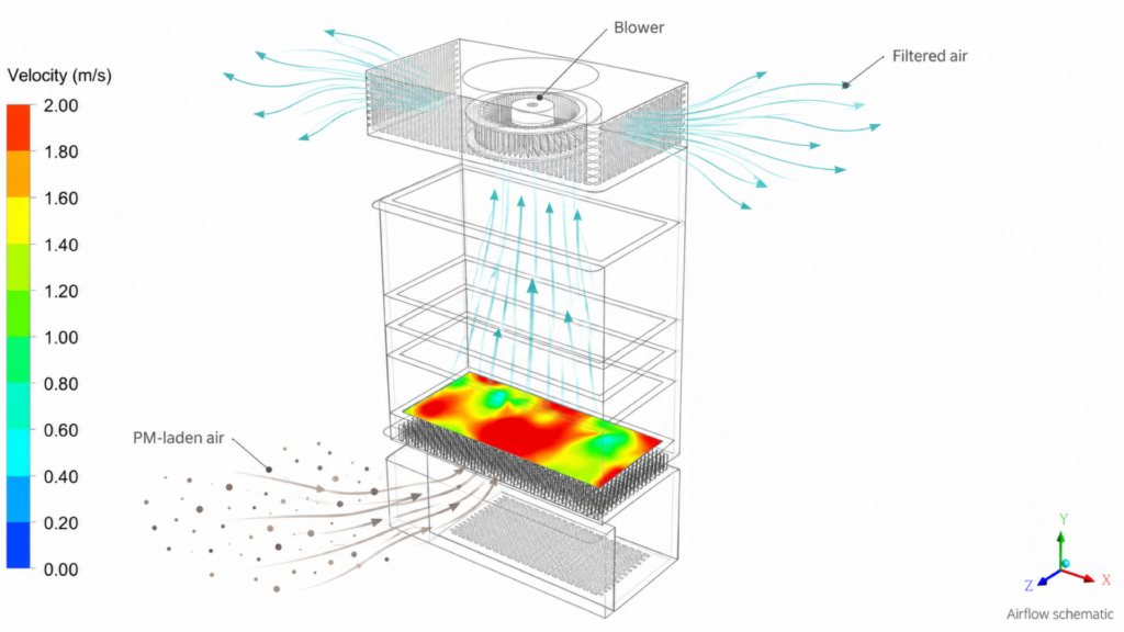
An air purifier can move air through its enclosure while distributing it unevenly across a filter. Some regions may receive more flow than others, and a single airflow value cannot show where that happens. Engineers need to understand the path from the inlet, through the filter stack, to the delivery vents.
In a Graphler Technology Solutions air filtration study, CFD revealed a clear difference between the pre-filter region and the main filter stages. The pre-filter showed an uneven velocity pattern, while the flow became more evenly distributed through the subsequent stages. This gave the design team specific regions to investigate.
Representing the airflow path
The evaluated unit included a fresh-air inlet, a honeycomb structure, a pre-filter, F9 and carbon filtration stages, an H13 HEPA filter, a fan region and delivery vents. The analysis considered a case with the recirculation vents closed.
Filters were represented using porous resistance based on the available pressure-drop data. This enabled the model to account for their influence on the flow through the enclosure without resolving every pore in the filter media. The CFD assessment then examined internal velocity patterns and the distribution across individual filter faces.
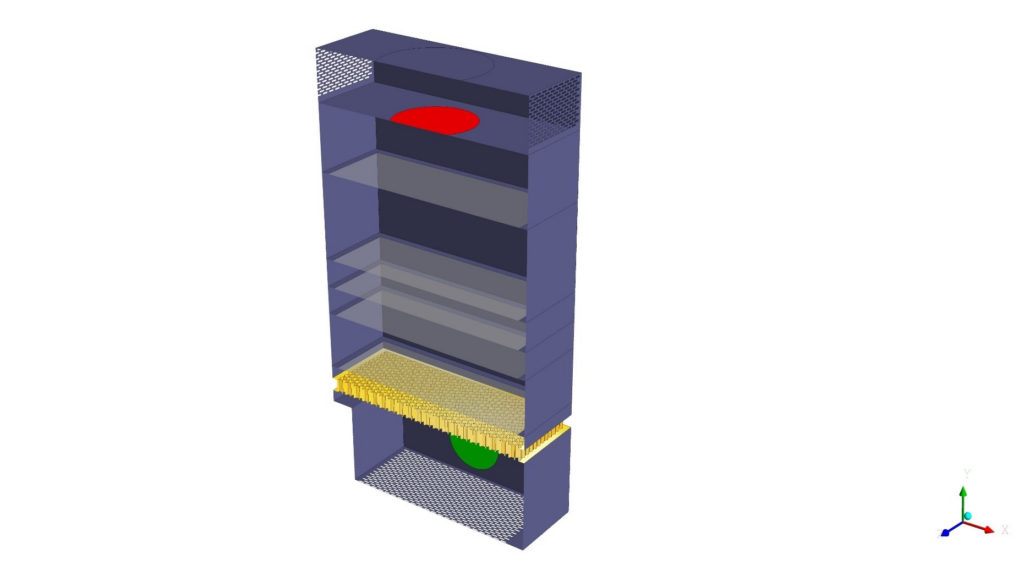
Figure 3. CFD geometry of the air filtration unit, showing the enclosure and internal flow path through the filter stack.
Locating the uneven flow
The velocity plots showed nonuniform flow near the inlet and pre-filter. The report described concentrations of velocity near the centre and sides as air approached the honeycomb, followed by an irregular pattern at the pre-filter face.
Farther through the unit, the F9, carbon and HEPA filter faces showed a more even distribution. After the HEPA stage, the flow became more disturbed around the extraction fan and delivery region. The study therefore identified different flow conditions in different parts of the same enclosure.
Reading filter face velocity alongside the contours
The pre-filter had a reported average face velocity of about 1.85 m/s. The main filter stages were approximately 1.3–1.4 m/s. These averages are useful, but the contour patterns explain how evenly the air reaches each face.
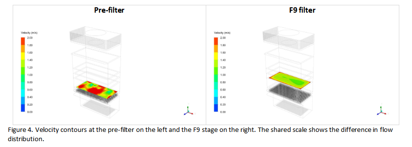
Figure 4. Velocity contours at the pre-filter on the left and the F9 stage on the right. The shared scale shows the difference in flow distribution.
| Region assessed | Average face velocity | Observed distribution |
| Pre-filter | About 1.85 m/s | Uneven |
| F9, carbon and HEPA stages | About 1.3–1.4 m/s | More evenly distributed |
For this configuration, the pre-filter region stands out as a candidate for further investigation. Changes to the inlet approach, available flow-development space or local flow guidance could be compared in a subsequent study. The present analysis identifies where to focus; it does not claim that a modified design has already been tested.
Understanding the noise assessment
The project also reviewed aeroacoustic contours. Higher acoustic activity was identified near the fresh-air entry and delivery vents, where the report associated it with disturbed flow. These locations offer a useful starting point for examining inlet and outlet geometry.
The acoustic scope covered flow-generated noise. It excluded mechanical noise from fan rotation and physical vibration, so the contours should not be read as a complete prediction of the finished product’s operating sound level.
Turning airflow findings into design priorities
This case shows why filter selection and enclosure airflow need to be considered together. CFD can distinguish an inlet distribution issue from conditions farther through the stack, helping a team choose which region to modify and which results to compare in the next iteration.
Airflow uniformity is one part of purifier performance. These results do not establish particle-removal efficiency, clean air delivery rate or filter service life. Those outcomes require the relevant filtration and product testing. The value of this study is its view of the internal airflow and the design questions it makes possible to investigate.
For a filtration unit or ventilation product, share the enclosure geometry, filter resistance data and intended operating conditions with Graphler. We can help define a CFD assessment of the flow distribution through the system.
Explore our CFD analysis services or discuss your project with Graphler. Email: info@graphlertech.com.